Hold Time Analysis in Vivado: Hold vs Setup Slack

1. Introduction

We’ve already discussed how to do setup analysis in Vivado in previous blogs. In this blog we’ll be looking at how to do analysis and interpret information provided by Vivado for hold analysis.

2. Hold Slack vs. Setup Slack

In setup analysis, the slack equation was:

\[\text{Slack} = \text{Required Time} - \text{Arrival Time}\]

For hold, it flips:

\[\text{Hold Slack} = \text{Arrival Time} - \text{Required Time}\]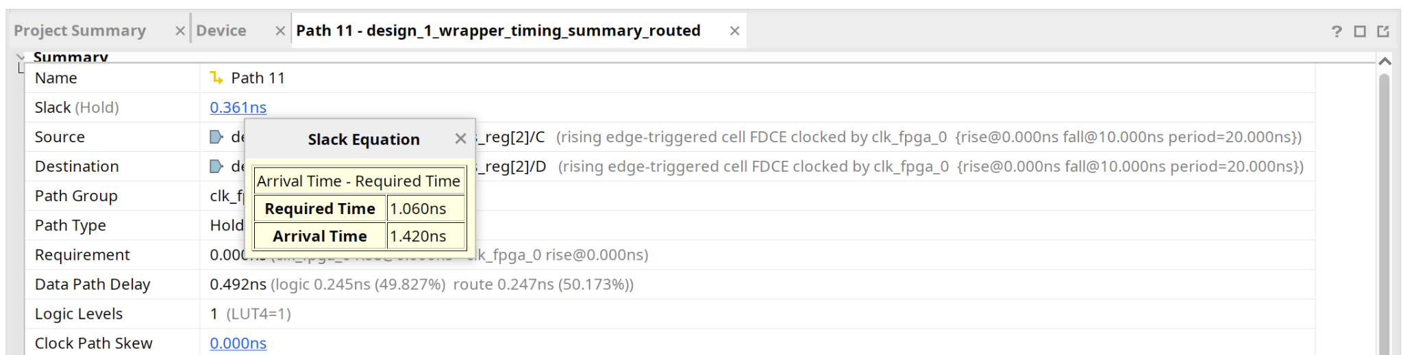

Figure 1: Hold slack equation in Vivado

For setup, data must arrive before the required time, i.e. data can take at max required time to arrive. For hold it’s the opposite: data arrival time must be greater than the required time, i.e. data must take time at least equal to required time to arrive. The data can’t change too quickly after the clock edges.

Another key difference is that in hold analysis, the source and destination clock edges are the same edge. In setup, the destination registers capture on the clock edge following the source clock edge, i.e. the next cycle. In hold analysis, both happen on the same edge.

2.1 Why is the Same Clock Edge Used?

Hold time basically asks: “After the clock edge, does the data stay stable long enough?”

Now the same clock edge that makes the destination register latch data also triggers the source register to release new data. So right after that edge, new data starts propagating through the combinational logic toward the destination. If the path is too fast, the data will reach the destination register before hold time window is complete.

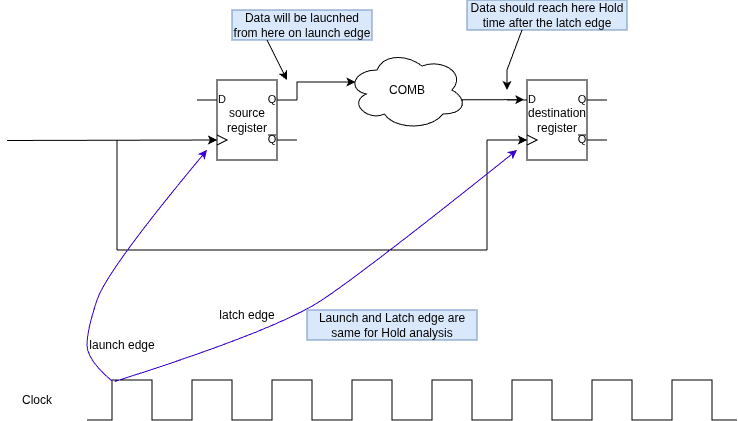
Figure 2: Same edge for launch and latch/capture edge

So, both arrival and required time reference the same edge because that’s the real scenario; one edge captures the current data initiating the hold window, while simultaneously releasing new data that might arrive too early.

3. Clock Delays in Hold Analysis

In setup, the tool uses:

• Max delay for Launch clock path → data gets out as late as possible
• Min delay for Capture clock path → capture edge arrives as early as possible, hence reducing setup slack.

For hold, it’s reversed compared to setup:

• Min delay for Launch clock path → data gets out as early as possible
• Max delay for Capture clock path → capture edge arrives as late as possible; we know data must not change “hold time” after the clock edge. So, if the clock edge arrives late, the data must remain stable for more time. I.e. the hold slack is reduced.

That represents the worst case: data arrives early while the hold window — the period during which data must remain stable — extends further in time, increasing the risk that new data arrives before the window closes.

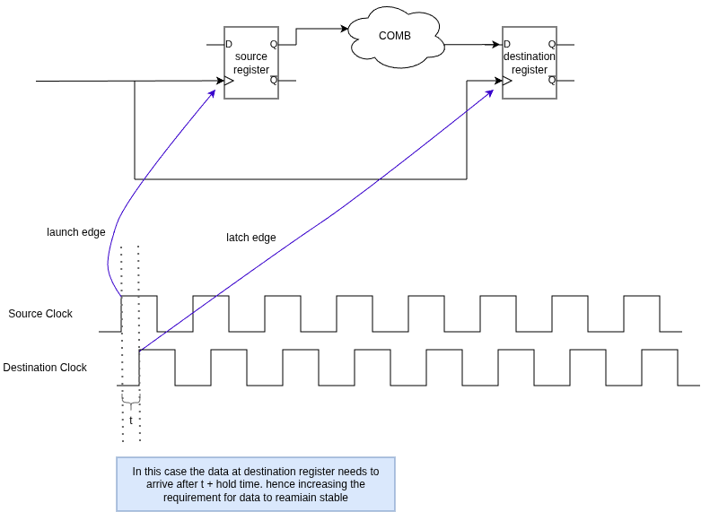
Figure 3: Launch and Capture Clock Path delay effect on Hold slack

Figure 3 shows the two clock waveforms for the launch and capture paths. These are not two separate clocks; it is the same clock drawn twice to illustrate that the signal takes different paths to reach the source and destination registers, which is why each path can have a slightly different delay.

4. Clock Pessimism Removal (CPR)

4.1 Why is CPR Subtracted for Hold but Added for Setup?

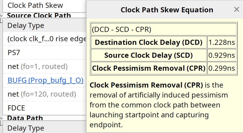
Figure 4: Clock skew equation for Hold analysis

First a reminder: the source and destination registers share the same clock path from the clock root up until the two paths diverge.

As discussed in section 3; the tool applies different delay corners to launch and capture clocks to model worst-case behavior. For setup analysis, it assumes the launch clock is late (MAX delay) and the capture clock is early (MIN delay). If part of the path is shared, that same segment is treated as MAX on the launch side and MIN on the capture side simultaneously; which cannot happen physically. This artificially makes the capture edge appear earlier than it really would be, reducing the required time and worsening slack. CPR corrects this by adding back the extra pessimism introduced on the shared segment.

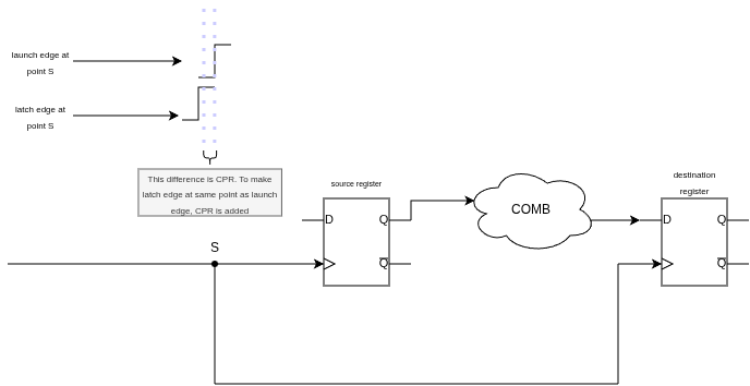
Figure 5: Setup Analysis; Pessimistic MIN/MAX Delays on Shared Segment; An earlier latch/capture clock arrival increases arrival Time, which reduces setup Slack.

Figure 5 shows how applying MIN and MAX delays to the shared segment simultaneously creates artificial pessimism that does not reflect physical reality.

For hold analysis, the corners are flipped: launch uses MIN delay and capture uses MAX delay. Now the shared segment is treated as MIN on one side and MAX on the other, making the capture edge appear later than reality and artificially inflating the required time. Since $\text{Hold Slack} = \text{Arrival Time} - \text{Required Time}$, an inflated Required Time directly reduces hold slack, so CPR removes this artificial reduction. In both setup and hold, CPR simply removes the fake delay difference created on the shared clock segment and pulls the required edge back toward physical reality.

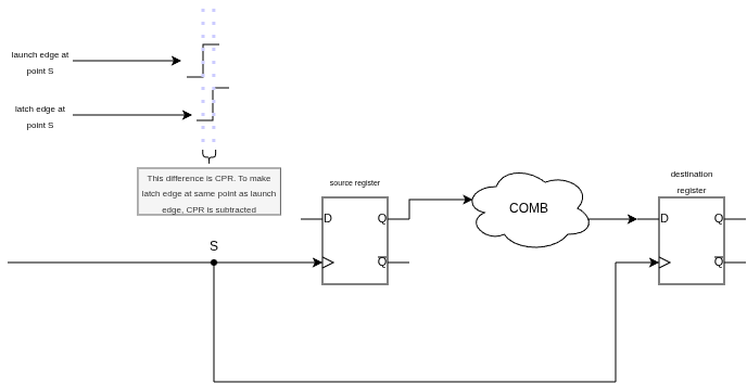
Figure 6: Hold Analysis — Pessimistic MIN/MAX Delays on Shared Segment; A later capture clock arrival increases Required Time, which reduces Hold Slack.

4. What’s Next

This wraps up our discussion on setup and hold time anaylysis in Vivado. Till now we have focused on reg-to-reg timing analysis. From next week we’ll start looking to pin-to-reg and reg-to-pin timing paths and analysis.

This is Part 3 of the Timing Analysis in Vivado series. Read Understanding FPGA Timing Analysis in Vivado: Part 1 and Understanding FPGA Timing Analysis in Vivado: Part 2 if you haven’t already.

← Previous Home Next →